Posted 7/21/96
Price–Earnings Ratios as Forecasters of
Returns:
The Stock Market Outlook in 1996
by Robert J. Shiller
The theory that the stock market is approximately a random walk does not look right at all: Figure 1 is a (log-log) scatter diagram showing for each year 1901–1986 the ratio of the real Standard and Poor Index ten years later to the real index today (on the y axis) versus a certain price–earnings ratio: the ratio of the real Standard and Poor Composite Index for the first year of the ten year interval, divided by a lagged thirty year moving average of real earnings corresponding to the Standard and Poor Index (on the x axis). Index values are for January, conversion of nominal values to real values is done by the January Producer Price Index. The variable shown on the x axis is publicly known at the beginning of each ten year interval. If real stock prices were a random walk, they should be unforecastable, and there should really be no relation here between y and x. There certainly appears to be a distinct negative relation here. The January 1996 value for the ratio shown on the horizontal axis is 29.72, shown on the figure with a vertical line. Looking at the diagram, it is hard to come away without a feeling that the market is quite likely to decline substantially in value over the succeeding ten years; it appears that long run investors should stay out of the market for the next decade.
Is this conclusion right? How can we reconcile it with the widespread public impression that the random walk hypothesis is at least approximately true?
Ratios as Indicators of Market Overpricing
The scatter diagram shown in Figure 1 (and in the subsequent figure) is unusual, in that the measures shown on both axes relate to the long run. Ratios of stock market indices to measures of fundamental value (such as earnings) as indicators of the outlook for the market appear to be most useful when they relate properly to the long run; this is the lesson of a number of recent papers. The denominator of the ratio should be some measure of long-run fundamental value, such as long-run earnings, and the outlook for the market that is to be forecasted should be a long-run one.
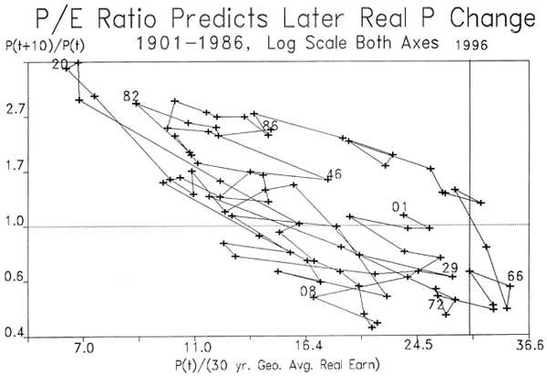
FIGURE 1
John Campbell and I studied the relationship depicted in the figure in a series of papers written in the late 1980s. The R2 in a regression of the scatter diagram shown in Figure 1, that is, of the log ratio of prices onto the log price earnings ratio, is 0.514, which means that over this interval from 1901 to 1986, more than half of the variance of the (log) price change could have been explained in advance by this simple ratio. There are some concerns about interpretation of this scatter, due to possible small sample effects, but the strength of the association seems so strong as to suggest that this relation is not consistent with the efficient markets or random walk model.
The ratio used here to predict the stock price changes, the ratio of real price to a thirty-year moving average of real earnings, tends to be higher than the conventional price earnings ratio because earnings tend to grow over thirty years, and so the denominator of the ratio tends to be low. Thus, the average ratio is higher than one might have expected, the average ratio over the sample shown is 18.28. Today, with a ratio of 29.72, well above average though not at record levels. The fitted value for today of the regression is –.479, implying an expected decline in the real Standard and Poor Index over the next 10 years of 38.07%.
The scatter diagram shown in Figure 1 is unusual in two ways: the price earnings ratio is defined in terms of thirty-year averages of earnings, rather than last year's earnings, and the interval over which real prices are forecasted is ten years, much longer than most are accustomed to.
The simplest and most widely used ratio used to predict the market is the price–earnings ratio. The use of one-year's earnings in the price–earnings ratio is an unfortunate convention, recommended by tradition and convenience rather than any logic. As long ago as 1934, Benjamin Graham and David Dodd, in their now famous textbook Security Analysis, said that for purposes of examining such ratios, one should use an average of earnings of "not less than five years, preferably seven or ten years." (p. 452) Earnings in any one year tend to be affected by short-run considerations, that cannot be expected to continue. In the present time, earnings have suddenly shot up in the last few years, bringing price–earnings ratios down dramatically, but it is doubtful that such sudden changes are meaningful. We extend our moving average even further than Graham and Dodd did, on the supposition that even more smoothing is advantageous, and Graham and Dodd didn't have the data then to make such smoothing possible.
We chose to represent long-horizon returns, of ten years, since that is what really matters to most investors, because there is so much interest today in long-term investing, and because there is recent evidence in the statistical literature that the long-horizon returns are more forecastable. This may be contrary to one's expectations; one might have thought that it is easier to forecast into the near future than into the distant future, but the data contradict such intuition. This forecastability of the market is not the kind of thing that will enable us to forecast that a crash is around the corner; it is forecasting gradual trends, analogous to forecasting the prospects for a city based on population trends, or forecasting the success of a university in terms of the number of young people who are enrolling.
Note that the apparent predictive relation is not really an artifact of the 1929 crash, as some might suspect. The year 1929 is not a real standout on the plot, and the postwar years 1972 and 1966 offer more dramatic support for the theory that price changes are related to price–earnings ratios. Neither is the 1987 crash of much importance to these results: the point corresponding to 1978 (ten years before our first post-crash observation here of January 1988) is not a standout on this plot. Our price–earnings variable is 11.12 in 1978, below the average of 18.28 in this data set, and the log price change from 1978 to 1988 is 0.57, somewhat higher than average ten-year log price change of 0.16, offering some mild support for our theory. The crash of 1987 itself actually works against the theory, since the model predicted an above-average increase in real stock prices over the ten-year interval 1978–88, and the crash served to make the increase less far above average.
Figure 2 shows a time-connected scatter diagram of the real (inflation corrected) gross return on the Standard and Poor Composite Stock Price index versus the same ratio of real price to the 30-year average of lagged real earnings. On this diagram, the relation looks even more striking, that is, the negative relation between price earnings ratio and subsequent return is stronger, more linear in appearance. The reason for the better fit in this relation is returns are affected by the price–earnings ratio in two ways: by the effect on subsequent price changes, as seen in Figure 1, and also by their effect on dividend yields. Times of very high price earnings ratios tend to be times of low dividend yields. The low dividend yield in such circumstances tends to persist for years, thereby contributing further to the low returns.
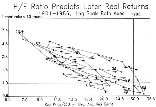
FIGURE 2
For forecasting three year returns Campbell and I [1988] achieved an R2 of 0.195 with this single forecasting variable alone; for forecasting ten-year returns, we achieved an R2 of .566. In contrast, if we used the simple log earnings price ratio as the independent variable, the R2 for forecasting three-year returns was only 0.090, and for forecasting ten-year returns was 0.296.
The additional nine year's data since our 1988 paper has been kind to our results: the R2 in a regression of ten-year real returns on our ratio of real price to thirty-year moving average of real earnings rises for the full sample to 0.624. By extending our data past 1987, we are able now to observe the ten-year interval starting in 1982, and the high ten-year returns predicted by the low ratio in 1982 is borne out well by the actual return.
If we substitute the January 1996 value for the ratio, that is 29.72, then the predicted log ten-year return is –0.06, virtually zero. Of course, this is not the same as the expected return. If returns are skewed to the right, as would be suggested by a lognormal distribution, then the expected return may be substantially higher. The lognormal assumption and our estimated regression model would imply that the expected return is exp(mean + variance/2) where mean is the expected log gross return and variance is the squared standard error of the regression: with these we come up with an expected total return over the succeeding ten years of .009, or about a tenth of a percent a year.
This forecastability in the market is not due to a market response to the forecastability of interest rates. Campbell and Shiller [1988] found that if one substitutes as dependent variable in the ten-year return equation the log of one plus the ten-year return on the standard and Poor Composite minus the log of one plus the ten-year return on investing in 4–6 month prime commercial paper, the results are virtually unchanged, the R2 in the regression is still 0.480. All of these results are statistically significant: using a Wald test that takes account of the overlapping observations of the dependent variable, we find that the significance level for the ten-year real return equation is 0.000; for the ten-year excess return equation it is 0.002.
Possible biases in the Relationship
Since the regressions have stochastic regressors, we have to expect some bias in the estimated coefficient. In simple terms, even if stock prices have no relationship at all to simple earnings, so long as earnings are smoothed enough to generate the price–earnings ratio, there will tend to be a negative correlation small samples between the price earnings ratio and the thirty-year average of earnings. The negative correlation arises primarily because the sample mean is estimated over the whole sample, and prices will naturally appear to be mean reverting to their sample mean, even if no true mean exists.
I did a simple monte carlo experiment to suggest how important such a bias might be. We generated 96 (annual) observations of a random walk (this number corresponding to the 96 observations 1901 to 1996 used to produce the 86 points shown in the scatter diagram in Figure 2), and regress ten-year changes in the random walk on its level at the beginning of the random walk. This regression shows a sort of limiting case of our story, in which earnings are so smoothed as to be a constant, and so that the earnings play no role in our analysis. In this monte carlo experiment, with 10,000 iterations, we found that the R2 did tend to be positive: the average R2 was 0.26. However, in these monte carlo experiments we achieved an R2 of .624 only 1.9% of the time; suggesting that the results are indeed highly significant.
In another monte carlo experiment I sought to represent the 30-year moving average of earnings as something other than a constant: we replaced it with a thirty-year moving average of lagged prices; this seemed like an interesting experiment, in that thirty-year averages of log earnings look fairly similar to 30-year averages of log price with actual data, up to an additive constant. In each iteration of the monte carlo experiment, a new 126-element (annual) random walk was generating, and for elements 31 through 116, a vector of subsequent ten-year changes was created, as the dependent variable. A vector of independent variable observations was taken by first creating the vector of elements 1 through 116, and then subtracting from each the 30-year average of lagged price. In each iteration, we regressed this dependent variable on the independent variable, and recorded the R2. In 100,000 iterations the average R2 was 0.124, far below what we have observed, and in only 0.26% of the iterations was the R2 greater than 0.62.
Possible Errors in the Index Used to Convert Nominal to Real Values
Note that our scatter diagram refers to real prices, real returns, and real earnings. It is important to couch our analysis in these terms, since we are concerned with real, not nominal, quantities. But, introducing indices of price inflation introduces the possibility of error.
The period around 1920 seems to have a lot of leverage, and is possibly accounting for too much of our fit. The behavior of our series around 1920 could possibly be an artifact of our price index, a producer price index, which may showed much more volatility around the 1920–21 recession than did other price indices.
Why Long Horizon Returns?
There is some popular confusion about the significance of this predictability in forecasting long-horizon returns. A source of concern that many people express is, if one-year returns are not significantly forecastable, why should the ten-year returns, which are just ten-year averages of the one-year returns, be significantly forecastable? The reasons for the greater power of the tests predicting ten-year returns are described in Campbell [1992]. A related confusion concerns the apparent random-walk property of one-year returns. How, some will ask, can it be that one-year returns are so apparently random, and yet ten-year returns are mostly forecastable? The answer is that it is known that stochastic processes that are near unit root for one-year intervals can be substantially forecastable over longer intervals. In looking at one-year returns, one sees a lot of noise, but over longer time intervals this noise effectively averages out, and is less important.
Warnings About the Above Analysis
The conclusion of this paper that the stock market is expected to decline over the next ten ears and to earn a total return of just about nothing has to be interpreted with great caution.
Our search over economic relations that us to study the price divided by 30-year moving average of earnings may have stumbled upon a chance relation with no significance. In other words, the relation studied here might be a spurious relation, the result of data mining. Neither the statistical tests nor the monte carlo experiments take account of the search over other possible relations.
It is also dangerous to assume that historical relations are necessarily applicable to the future. There could be fundamental structural changes occurring now that mean that the past of the stock market is no longer a guide to the future.
References
Campbell, John Y., and Robert J. Shiller, "Stock Prices, Earnings, and Expected Dividends," Journal of Finance, 43(3): 661-76, July 1988.
_____, "The Dividend Ratio Model and Small Sample Bias: A Monte Carlo Study," Economics Letters, 29: 325-31, 1989.
Graham, Benjamin, and David L. Dodd, Security Analysis, First Edition, McGraw Hill, New York, 1934.
Helwege, Jean, David Laster, and Kevin Cole, "Stock Market Valuation Indicators: Is This Time Different?" Federal Reserve Bank of New York Research Paper No. 9520, September 1995.
© 1996 Robert J. Shiller
Raw data used to produce
figures are also on this web site.